Background
During the fall 2020 semester, I did a fair amount of research into mainstream cryptocurrency such as bitcoin as well as more contemporary privacy-coins such as monero. In addition to reading about, playing around with, and writing code to implement the different functions of these cryptocurrencies, I developed a variety of software projects. One of the products of my research is a bitcoin trading bot written in python.
Note: as I have not released the final version of this software in any capacity, no source code will be provided or linked.
Theory
This trading bot uses moving averages to determine whether a cryptocurrency is likely to increase or decrease in value. An ‘n’-day moving average is simply the average of an asset’s value over the past n days. Studying assets’ moving averages over different windows of time is a fundamental tool used in both the cryptocurrency and stocks trading worlds.
A chart displaying moving averages looks like this:
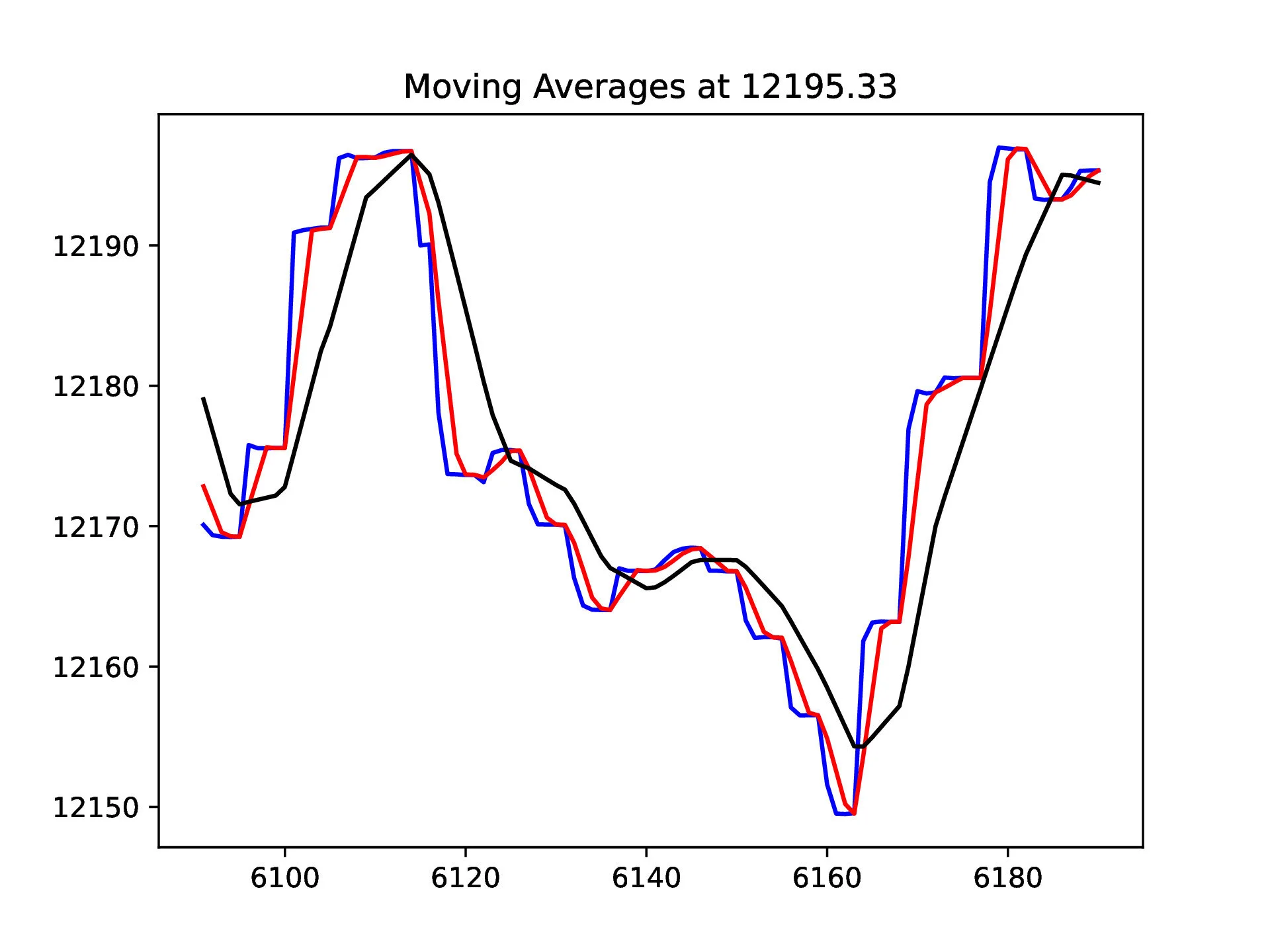
Chart 1A
The blue line represents the asset’s price (BTC in this case), while the red line is an arbitrary moving average m1 and the black line is another arbitrary moving average m2. In this case, the window for m2 is larger than that of m1, which one can tell from looking at the figure. The red and black curves follow the general shape of the blue curve, but lag behind and display smoother features. By studying different moving averages of an asset over time, we can gain a good idea of when its value will increase or decrease.
A basic trading algorithm
Using moving averages, we can design a basic algorithm that trades the asset every time the faster moving average (m1, red) crosses over the slower one (m2, black). Whether the program will buy or sell the asset depends on the time rate of change of the faster moving average, m1. If m1 is increasing at its point of intersection with m2, the program buys, and if it is decreasing at its point of intersection, the program sells.
We can visualize this strategy by marking these points on the previous chart (1A) to create chart 1B (right). The green circles denote where this algorithm would buy, and the green circles denote where it would sell. We will call these points ‘signals’, as they indicate that the program should perform a certain action. As we can see from taking a brief look at chart 1B, this strategy performs fairly well, buying low and selling high, with our simple strategy being able to correctly predict major fluctuations in value.
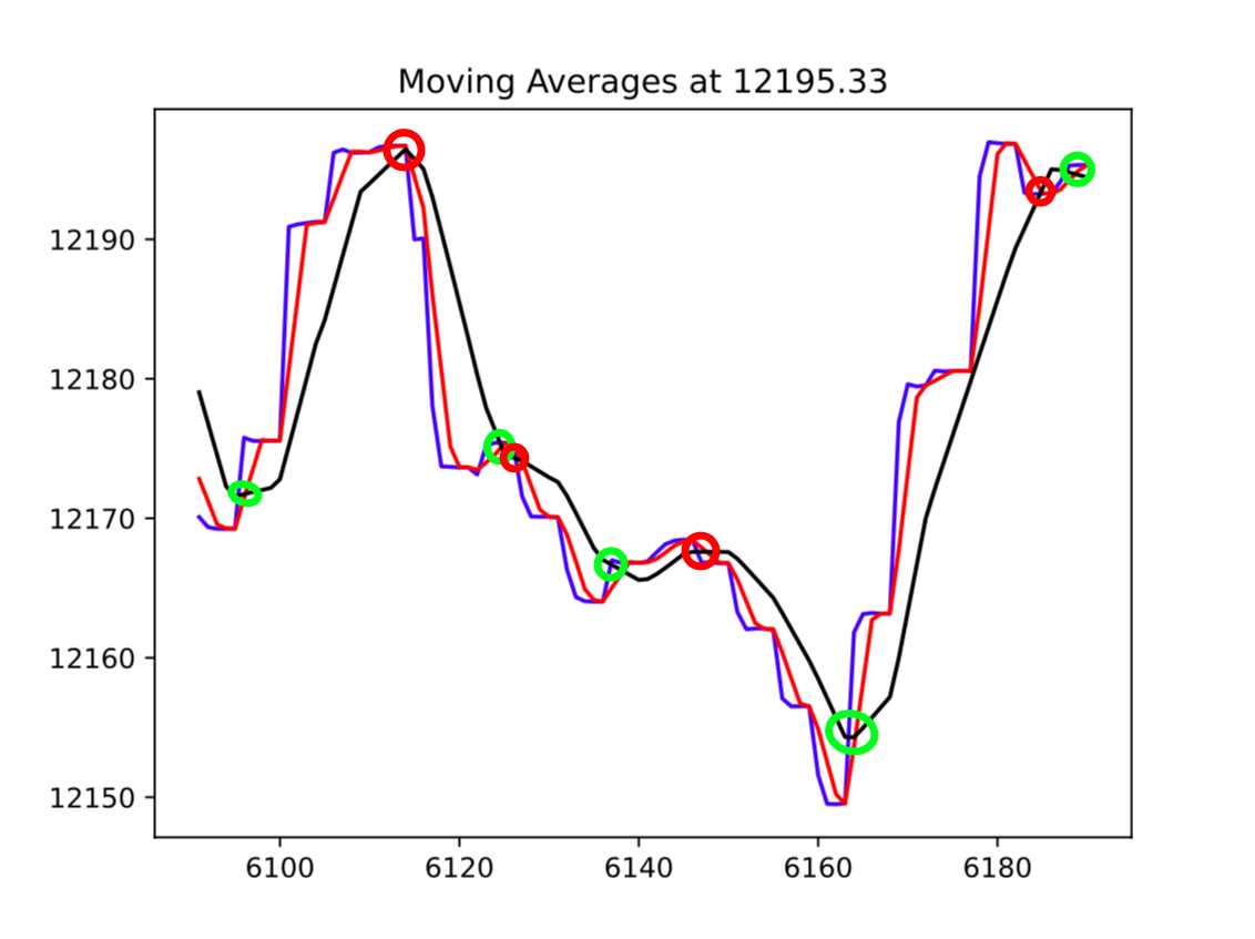
Chart 1B
Limitations and false signals
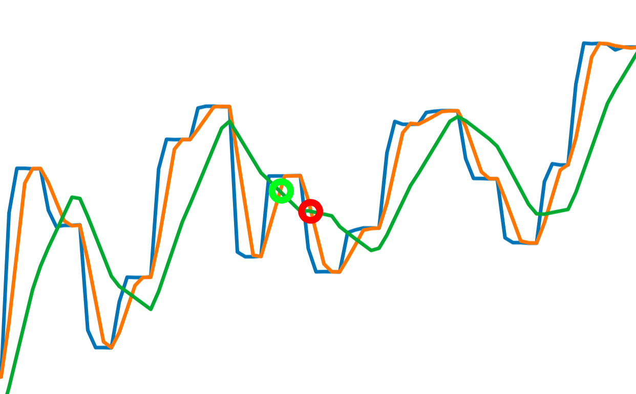
Chart 2
Now, if predicting value fluctuations were that easy, we'd all be millionaires. The truth is that the high prediction accuracy depicted by figure 1 is not the norm, and, if this algorithm runs for long enough it will not generate any notable increase in portfolio value.
Luckily, we can apply some more math in order to increase the profitability of this algorithm. First off, we want to make the algorithm aware of ‘false signals’, or false indications that an asset’s value will increase or decrease. Take, for example, chart 2, which shows a similar layout to chart 1, besides being zoomed in. In this chart, blue is the price of BTC, orange is the ‘fast’ moving average m1, and green is the ‘slow’ moving average m2. A false signal is generated when m1 crosses m2, but then changes direction and crosses m2 again in the opposite direction without the asset price moving sufficiently up or down. A false signal is indicated on chart 2.
Identifying false signals With moving average analysis
Identifying false signals in a simple, reliable, and computationally quick manner was something that I put a lot of thought into while developing this software. After hours of analyzing, transforming, and manipulating data from charts, I realized that by combining data from moving averages of different size from a dataset at a singular point in time, I could predict the direction of an asset’s value fluctuation to a high degree of accuracy.
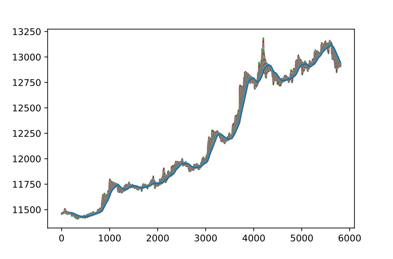
Chart 3
This detection algorithm is based upon the fact that moving averages calculated over different windows of time (ie 1 day vs 30 days) provide an indication of how the asset’s value will fluctuate over a specific time frame. If we plot a variety of moving averages on a single chart, we get a result that looks like chart 3, where the blue curve indicates the asset’s value and the blue/red curves represent moving averages of varying ‘n’.
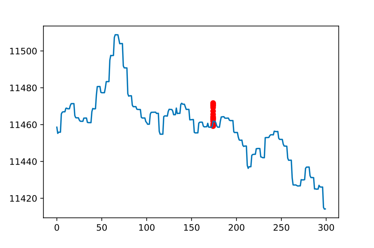
Chart 4
Plotting these points at only one value in time, such as in chart 4 gives a much clearer picture. Each red dot represents the value of some moving average at that point in time. Plotting these points against time is meaningless, but if we transform these points into the n dimension (plot each value of n against the value of its corresponding moving average), we get something like chart 5, which is more meaningful.
The data displayed in chart 5 shows us how moving average values vary depending on their n-value, which gives an indication of the stability of the asset as well as a better idea of how its value is changing in the long-term. For example, if the points in chart 5 were spread out over the y-axis and did not form a clear trend, it would indicate that the asset is unstable, as its value in the short-term varies vastly from the trend of its value in the long-term. Since the points in chart 5 form a clear trend, we can assume that the movement in the asset’s price was reasonably stable over the period of study.
By determining a line of best fit for the values plotted in chart 5 using the least squares method, we can quantify the overall trend of the asset’s price (indicated in chart 5 by the blue curve). Additionally, the volatility of the asset can be gauged from the correlation coefficient of the calculated linear fit. Incorporating this new data into our trading program allows it to detect and avoid false signals using the following logic: If the sign of the correlation between an asset’s moving average window size n and the value of said asset’s n-period (days, minutes, etc..) moving average are opposite, then it is a false signal.
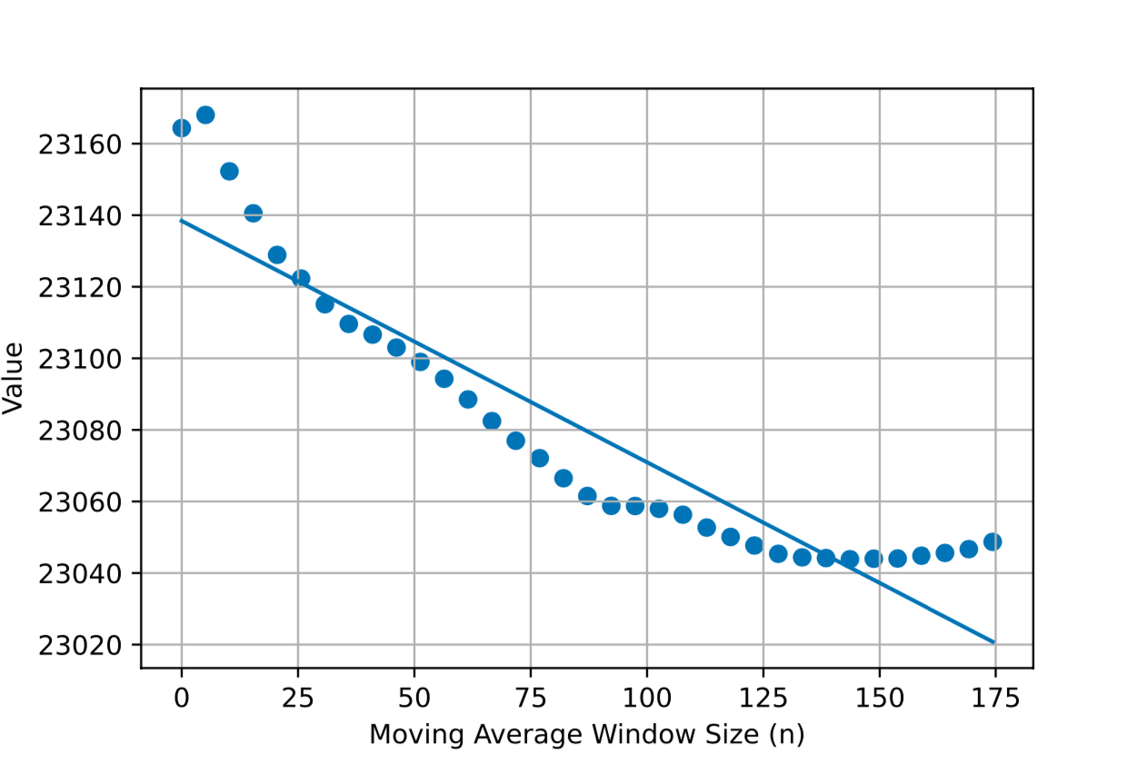
Chart 5
Basically, if the detected signal is not corroborated up by the overall trend of the data, such as the example shown in chart 2, then it will be ignored by the algorithm. Additionally, the asset’s calculated stability can be used to modify the program’s detection parameters on-the-fly so that it adapts to the current behavior of the market. For example, if an asset is deemed to be currently unstable, then the sensitivity, determined by the difference in n value between m2 and m1, will be decreased in order to respond to quicker and more vigorous price fluctuations.
simulated data and Results
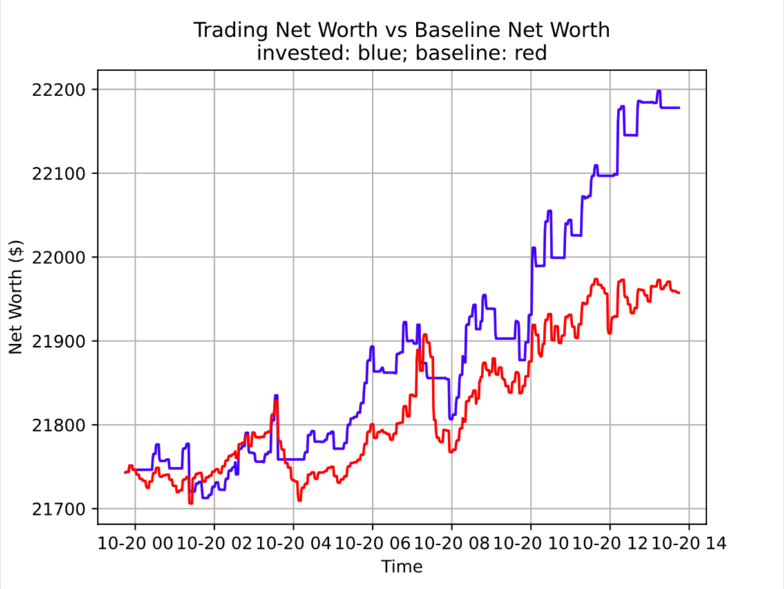
Chart 6
In order to test my trading algorithm, I wrote a python class to simulate both a USD and bitcoin wallet. This would allow the program to ‘paper trade’, or simulate a trading strategy in real time without using any funds. I let my program paper trade BTC for around 14 hours and tracked the net worth of its portfolio compared to BTC’s price. The results are shown in chart 6 (left). My program outperformed the market over the majority of the trial period, out-performing the market by approximately 1.002%. Obviously, the period of study in chart 6 is not large enough to make any real assessment of the program’s performance. I conducted a variety of trials over a few weeks, and got very promising results. On average, my program increased the net worth of its portfolio by around 1% every twenty-four hours. Though this figure is an average, 1% per day, assuming the profit is reinvested in the portfolio, works out to a yearly increase of 3678.3%, or just over a 36-fold increase in value. By comparison, the average stock market return over the past twenty years (before inflation) has been around 10%.
Trading real crypto algorithmically
These astronomical simulated returns mean nothing if we cannot actually trade the asset that we are studying. I researched a variety of cryptocurrency brokers, looking for one with a python API, and, most importantly, low enough fees. Since this program works by making a large amount of trades over a short period of time, it is critical that the profit from each trade be larger than twice the brokerage fee. For example, to buy and sell 1 BTC on Binance we would have to pay 0.75% on each transaction, or a total of 0.015 BTC. If this trade only profits by 0.5%, we will be losing money overall.
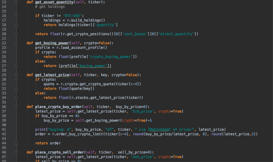
I ended up choosing Robinhood for this project as they do not collect a commission on crypto trades, and their day-trading restriction does not apply to crypto. Additionally, they have an API with multiple community-made python wrapper libraries which made integrating real trades into my project much easier. The final result is a program that trades cryptocurrency (Robinhood only supports bitcoin and ethereum at the time of writing) and outperforms the market to a significant degree.
Shortcomings and Roadmap
The downside to using Robinhood to trade crypto algorithmically is that, while they do not charge commission, they implement a spread fee such as a foreign exchange broker would. A spread is the difference between the price a buyer is willing to buy an asset for (bid price) and the price a seller is willing to sell an asset for (ask price). Spreads on crypto are often around $0.01 or so, however Robinhood pads out their bid-ask spreads to a larger value and pockets the surplus between their reported bid/ask price and the real bit/ask price. This creates a ‘spread fee’, a concept is explained in much more detail here. Since my program places limit orders at the time of transaction (market orders on Robinhood are often fulfilled at a higher/lower price than expected, the width of the spread means that my order has a larger chance of remaining unfulfilled, especially if the price fluctuates dramatically. This essentially stops the program from working, as the funds for the unfulfilled order are set aside until it is fulfilled or cancelled. Additionally, it will take more in-depth analysis and live trials to determine whether my program is able to out-perform Robinhood’s spread fee, as it varies from trade to trade.
In order to make sure orders are fulfilled, I could implement an auto-cancel timer on each placed order. The spread fee issue is more nuanced and will require live trials, though if my program places limit orders ahead of what it predicts the market will do (assuming it is correct), I will be able to avoid the spread fee. The downside to this is that these orders will have less of a chance of being filled if they are offset from the current price by some amount. Since this program relies on its ability to trade very quickly and with high frequency, reducing the trade frequency in this way would also reduce profitability.
This is a project that I intend to continue and hopefully profit from once I have time to continue developing it.